
Summary
- Oil production continues to eclipse record highs on a weekly basis despite the oil rig count declining 49% since October.
- A single oil-well declines exponentially up to 75% in its first year of production. However, in a process known as Convolution, older wells buffer the rapid decline from new rigs.
- This article provides a comprehensive analysis of principles behind oil drilling and production, applies it to the current crude oil climate, and predicts future production, rig counts, and oil price.
- Based on my analysis, I remain short-term bearish but long-term bullish on the commodity. My trading strategy based on this analysis is discussed in detail.
by Force Majeure | Seeking Alpha
On Friday, March 20, Baker Hughes (NYSE:BHI) reported that the crude oil rig count had fallen an additional 41 rigs to 825 active rigs. This was the 15th straight week and 25th out of 26 weeks that the rig count has declined. Active oil rigs are now at the lowest level since the week ending March 18th, 2011 and total drilling rigs (oil + natural gas) are the fewest since October 2009. Overall, the oil rig count is down 49% in the 23 weeks since peaking in October. Nevertheless, in its weekly Petroleum Report, the EIA announced last Wednesday that domestic oil production set yet another record high of 9.42 million barrels per day. Since the rig count peaked the week of October 10, 2014 and began its subsequent collapse, oil production has climbed 460,000 barrels per day, or 5.2%. This continued increase in production in the face of a plummeting rig count has confounded journalists, flummoxed investors, and inflated supplies to record highs leading to a continued slump in oil prices.
The two main questions on traders’ minds are 1) why is oil production still at record highs five months after the rig count started dropping? And 2) when, if at all, will oil production begin to fall and how far will it fall? This article provides a comprehensive analysis of the principles behind the relationship between oil drilling and production, applies it to the current crude oil climate, and predicts where both production and the rig count will go in the coming year.
Before we discuss the real-world oil production and drilling situation – an extremely complex picture with over 1 million rigs producing oil – let’s look at a simple, hypothetical situation. The first key point is that once an oil well is drilled, its production is not constant. In fact, production not only begins to decline almost immediately, it does so in an exponential fashion. After analyzing production curves from multiple wells, I will be estimating weekly oil production from a single oil well by the following equation:
Equation 1:
Daily Oil Production From Single Well = (Initial Daily Production)/(1+ (Week # from start of production*K)
Where K is a constant equal to 0.06
When graphed using a well that initially produces 1000 barrels of oil per week this equation is represented by Figure 1 below:
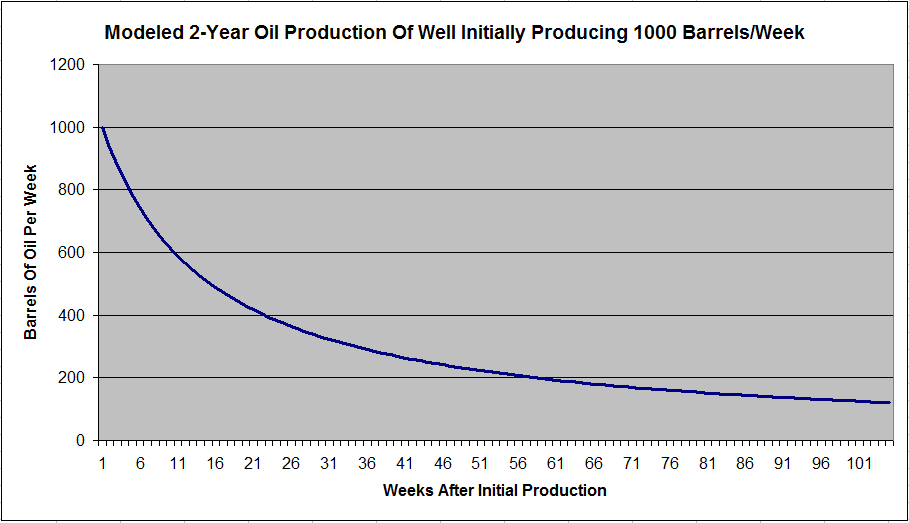
Figure 1: Crude oil production curve of single, hypothetical well showing exponential decay.
There are two take home points to note from this chart. First, initial decay is very rapid, with weekly production declining by about 75% after 1 year. Second, after the initial rapid decay, production declines much slower and becomes approximately linear with decay rates of 5-10% per year. Although this graph ends after 2 years or 104 weeks, production continues slowly and steadily beyond 5 years.
Figure 1 represents production from a single well. What happens when we add multiple wells over a period of time? The process by which multiple functions – in this case, oil wells – are added over time is known as Convolution. As noted before, even after an oil well has been active for many years, it is still producing a small volume of oil, a fraction of its initial output. However, there are a LOT of these old, low-output rigs – over 1.1 million in fact. When the number of drilling rigs decreases – thus reducing the number of new wells that come into the service – the old, stable wells plus the production from the declining number of new wells is initially enough to buffer the decline in rig count and net output will continue to rise.
Let’s illustrate this with a simple example. Imagine a new oil field monopolized with a single company that owns 30 oil rigs. The company adds five new rigs each month. Each rig is able to drill 1 new well per month. After six months, the company has deployed all of its rigs to the field. Unfortunately, shortly thereafter the company encounters financial difficulties and is forced to withdraw rigs at a rate of 5 per month until zero remain drilling. Figure 2 below compares active drilling rigs and total wells in this field.
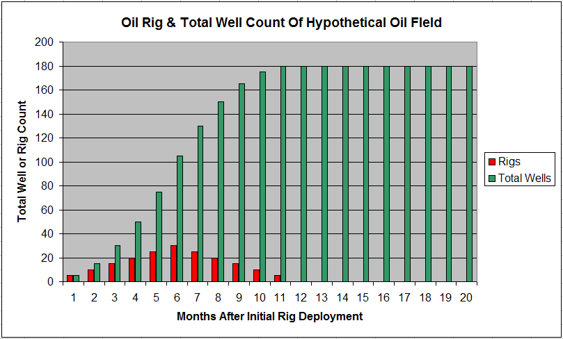
Figure 2: Rig count and total well count of hypothetical oil field
Note that after the rig count peaks and begins to decline, total wells continue to increase before ultimately peaking at 180, where it remains for the remainder of the 20-month period.
Each well initially produces 200 barrels of oil per day and declines according to Equation 1 and the chart in Figure 1. Figure 3 below shows total oil field production overlaid with the total rig count of the field.
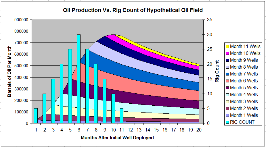
Figure 3: Oil Production from hypothetical oil field illustrating how crude oil production can continue to climb despite a sharp reduction in the rig count due to convolution.
Oil production initially climbs rapidly as more rigs are added to the field, reaching 500,000 barrels per month by the time the rig count peaks after 6 months. However, even though the rig count declines to zero six months later, total production continues to increase and peaks at 770,000 barrels per month in month 10 – 4 months after the rig count peaked. Production then begins to decline, but slowly. Even by month 20 after the rig count has been at zero for eight months, production has only declined by 33%.
This is obviously a simply, insular example, but it illustrates several important points. First, there is a delay between when the rig count peaks and when production begins to decline as the combination of old, accumulated oil wells and the continued addition of new wells by the declining rigs is sufficient to coast production higher initially. Second, even when production begins to decline, it is blunted, with production declining a fraction of the actual reduction in rig count. For those interested, the Following Article delves into these principles further and provides useful insight.
Let’s now apply these principles to actual domestic oil production. Before we can set up the model, there are three baseline metrics that need to be established: 1) Rate that rigs drill a well, 2) Time between initial spudding of a well and when it begins production, and 3) Initial production rate of new oil wells.
The EIA has released well counts on a quarterly basis for the past two years. Their data shows that the ratio of new wells to rigs has increased slowly from around 4.75 per quarter in 2012 to 5.3 per quarter in 2014. This equates to about 0.4 wells per week per rig presently. For the model, I used a linear reduction in drilling efficiency with drilling rates down to 0.3 wells per week per rig in 2006.
It takes 15-30 days to drill a new oil well. Once the hole is dug, the well must be completed. It typically takes another week for the rig to be removed and new equipment to be set up. A further week is devoted to hydraulic fracturing. Initial flow back and priming of production takes place over the next 3-4 days. Over the final week, the well is primed for continuous production including installation of tank batteries, the pump jack, and assorted power connections. The well is then connected to the pipeline and permanent production begins. Thus, it takes roughly two months from initial spudding of the well to when it begins production. However, once a well is completed it does not always begin to produce immediately and may not do so for up to six months.
Initial oil production rates have increased markedly over the past decade as drilling technology has improved. The EIA released the chart shown below in Figure 4 showing yearly initial production rates in the Eagleford Shale.

Figure 4: Yearly production rates in Eagleford Shale Formation showing rapidly increased initial rates of production 2009-2014. (Source: EIA)
Initial rates increased from less than 50 barrels per day (or 350 per week) in 2009 to nearly 400 barrels per day (or 2800 per week) in 2014. Note that the decay rate has also increased such that by 2-3 years, all wells are approaching the same output despite the significant differences in increased production. This is a relatively new oil formation and older formations produced more oil initially prior to 2010. For my model, I assumed initial production of 2625 barrels of oil per well per week in 2014-2015 with initial production declining to 1400 barrels per well per week in 2006.
Using this data and the methodology discussed in the example above, a modeled projection of U.S. oil production is created dating back to 2006. This data is shown in Figure 5 below and is compared to actual oil production, calculated on a weekly basis. My preferred unit of time is 1 week as this is the frequency that both the rig count and oil production numbers are released.

Figure 5: Projected oil production based on my model vs. observed crude oil production vs. Baker Hughes Rig Count [Sources: Baker Hughes, EIA]
Overall, this model accurately projects oil production based on active drilling rigs. Between 2006 and 2015, the average error was 88,000 barrels per day, or 1.2%. Over the past six months, this error has averaged just 44,000 barrels per day. The model correctly shows production continuing to increase despite the sharp reduction in active drilling rigs. It is interesting to note that the largest deviation between projected oil production and observed production occurred in late 2009 and early 2010, or shortly after the rig count bottomed out from the previous oil price collapse. The model predicted that oil production would decline somewhat while actual production actually just leveled off before beginning a new rally once the rig count rebounded later in 2010.
This model can be used to project how oil production might behave heading into the future. To do so, we must make assumptions about how the rig count might behave heading into the future. First, let’s pretend that the rig count stays unchanged at 825 active oil rigs for the next 1 year. Figure 6 below projects crude oil production to 1 year.
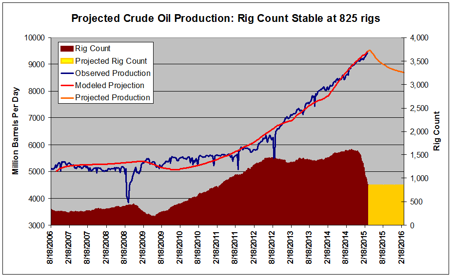
Figure 6: Projected oil production based the rig count remaining unchanged at 825 [Sources: Baker Hughes, EIA]
Using this projection, crude oil production will peak during the week ending April 10 at 9.51 million barrels per day and then begin declining. By next March 2016, production will have declined to 8.68 million barrels per day, down 9.5% from the projected peak. Again, this goes to show the buffering capacity of older rigs, given that a sustained 50% reduction in the rig count results in a comparatively small <10% decrease in output.
Two qualifying notes are necessary. This model shows a relatively short period of time between production plateauing and production beginning its decline. 1) Given that this model assumes all completed wells are producing oil within 3 months of spudding, it is certainly possible that the production curve may flatten out for a longer period of time due to additional completed wells that have been idle are slowly hooked up to pipelines over the next several months. 2) This model also makes the assumption that all rigs produce oil equally. If rigs drilling less-productive oil fields have been selectively retired while those drilling richer fields have remained active, the rate of decline will similarly be slower and less than projected.
The most recent historical comparison to the events currently unfolding took place in 2008-2009 following the collapse of oil from record highs during the great recession from a high of $146/barrel to near $30/barrel. The rig count during that event was likewise slashed by 50% before rapidly recovering when prices rebounded. However, this is not an apples-to-apples comparison since drilling technology has changed substantially – decline rates are much more rapid, initial production is nearly double that in 2008, etc – and inferences cannot necessarily be made about the future of production. However, let’s assume that the current rig count follows a similar trend. If so, the rig count will slow its descent and bottom out in roughly six weeks near 760-780. If the rig count follows the trend seen in 2009, the count will then rapidly rise and will reach 1330 by this time next year. Production will again peak during the week of April 10, before declining. Production will bottom out in late October near 8.9 million barrels per day, down just 6.3% from its peak before again increasing late in the year.
However, the decline in oil in 2008-2009 was based more on the combination of a bubble bursting and a slumping economy than fundamental forces while the current slump is predicated on a supply/demand mismatch. I expect this will keep prices and rigs down significantly longer than in 2008-2009. Let’s amplify the 2008-2009 rig count curve and project instead that rigs bottom out near 730-750 and that the rate of recovery is roughly half that of 2008-2009 with total rigs at just 950 this time next year. Using this model, production will continue to slowly decline through the New Year and flatten out near 8.7 million barrels per day by March 2016, down 8.4% from the peak. I believe that this is a more realistic model for crude oil production. This projection is shown below in Figure 7.
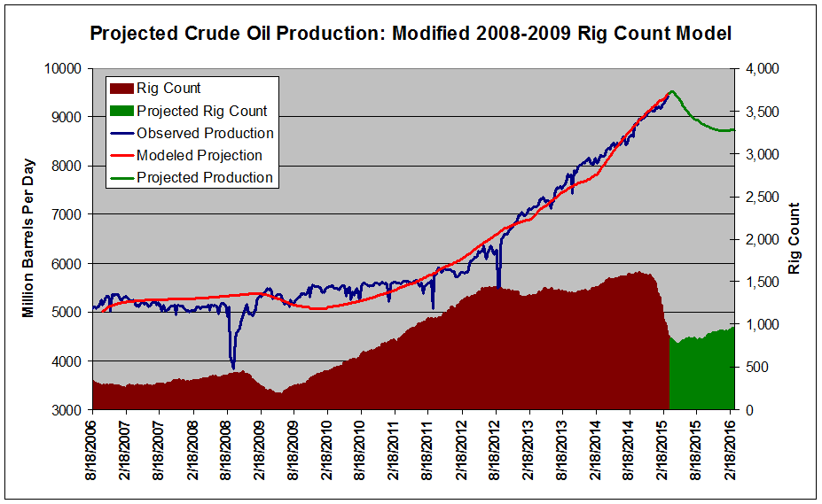
Figure 7: Projected oil production based on 2008-2009 rig count [Sources: Baker Hughes, EIA]
What does this mean for the supply/demand situation? As I have discussed in my previous articles, crude oil supply and demand are severely mismatched. This has led to oil inventories skyrocketing to a record high of 458 million barrels, a huge 98.7 million barrels above the five-year mean for March. Applying the projected production curve shown in Figure 7 to crude oil storage yields some surprising results. Even with just an 8.7% reduction in supply, the inventory surplus will narrow markedly. These results are shown below in Figure 8, which compares the five-year average storage level and current and projected storage levels. Note: These projections assume that total imports will remain flat and that total demand will follow the five-year average.
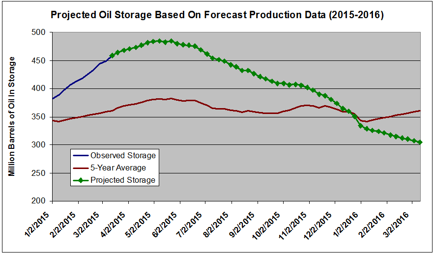
Figure 8: Projected crude oil storage based on projected oil production data vs. 5-year average [Source: EIA]
While the rig count continues to climb and then plateaus, I expect that the storage surplus will continue to widen with total inventories approaching 500 million barrels by early May. However, as production drops off, the inventory surplus begins to decline. By the last week of 2015, total supply has declined by 4.7 million barrels per week and projected inventory levels cross the five-year average for the first time since October 2014. Should the rig count begin the slow rise that is projected, by March of 2016, total storage levels will be 50 million barrels BELOW the five-year average. Even if the two qualifying statements discussed above verify or the rig count rises more rapidly than projected, I expect that, based on the drop in rig count already, crude oil inventories will be at or below average this time next year.

What does this mean for crude oil prices? There is a chicken and egg situation going on here. This article makes references to the rebound in rig count after bottoming out in the next month or two. This, of course, is predicated on a rise in price to make drilling again profitable. Without a rally, the count will continue to fall or, at the very least NOT rise, putting further pressure on supply and down-shifting the projected production curve further, making it more likely that prices will THEN rally. Until they finally do. One way or another, I do not see how crude oil can remain priced at under $45/barrel for longer than a few months. Something has to give. Drilling technology is simply not yet to the point where this is a profitable price range for the majority of companies.
Given that these projections show production increasing through early April, I would not be surprised to see continued short-term pressure on oil prices. As I discussed in My Article Last Week, storage at Cushing, the closely watched oil pipeline hub, continues to fill rapidly and threatens to reach capacity by early May. I would welcome such an event, as crude oil would likely drop under $40/barrel presenting an even better buying opportunity. I therefore maintain a short-term bearish, long-term bullish stance on oil.

My favorite way to play a rally in oil is to short the VelocityShares 3x Inverse Crude Oil ETN (NYSEARCA:DWTI) to gain long exposure. This takes advantage of leverage-induced decay to at least partially negate the impact of contango on the ETF. The United States Oil ETF USO), on the other hand, is intended to track 1x the price of oil and leaves an investor directly exposed to contango, which is now 15% over the next six months. The same applies to the VelocityShares 3x Long Crude Oil ETN (NYSEARCA:UWTI), except that exposure to contango is now tripled to 45%.
The advantage to USO is in its safety. A short position in DWTI theoretically leaves an investor open to infinite losses should the price of oil continue to drop. Further, shares must be borrowed to short, which can cost 3-5% annually depending on the broker. And if, once a trader has a position, these shares are no longer available, the position can be forcibly closed at an inopportune time. A slightly less risky position would be the ProShares UltraShort Bloomberg Crude Oil ETF (NYSEARCA:SCO) that is more liquid and less volatile.
For this reason, I started a small position in USO on Thursday at $16.05 when oil erased its post-Fed Remarks gains from Wednesday. This position is equal to just 2% of my portfolio. I will add to my USO position once oil breaks $45/barrel and then again should the commodity break $42/barrel for a total exposure of 6% of my portfolio. Should oil continue to decline to under $40/barrel, I will begin to sell short DWTI at what I assume to be a safer entry point until 10% of my portfolio is allocated to oil ETFs.

Should oil rebound, I will look to take profits. Once the rig count bottoms, I will begin taking profits once oil reaches $50/barrel. I will selectively sell USO initially. I prefer to close out the position most exposed to contango initially in the event that oil reverses and I would otherwise be stuck holding it for an extended period of time. I will then close out DWTI if and when crude oil again reaches $60/barrel. While I believe that oil may ultimately see higher prices, I am concerned at the speed at which rigs may be re-deployed once drilling again becomes profitable. I believe that this will keep oil under $70/barrel for the foreseeable future and will look to exit prior to this level.
In conclusion, an oil production model based on 9 years of domestic production and rig count data is used to project oil production for the past 1 year. This model suggests that oil will bottom around the week ending April 10. However, this is just a modeled projection and the actual peak in production will depend on nuances in drilling discussed above. Nevertheless, I believe that the peak in oil production will represent a significant psychological inflection point and that crude oil is poised for a rally once production begins to roll over.
