by Donald Van Deventer
Summary
- Wm. Mack Terry explained the basics of how rates impact bank stocks at Bank of America in 1974. Net income goes up, margins go up, and stock price goes down.
- We value a bank by replication, assembling a series of Treasury securities with the same financial characteristics as a bank. All of Mr. Terry’s conclusions are correct.
- A more technical analysis and references are provided. Correlations with 11 different Treasury yields are added in Appendix A. Finally, a worked example is given in Appendix B.
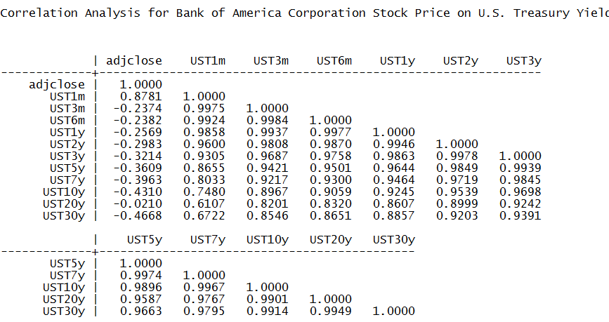
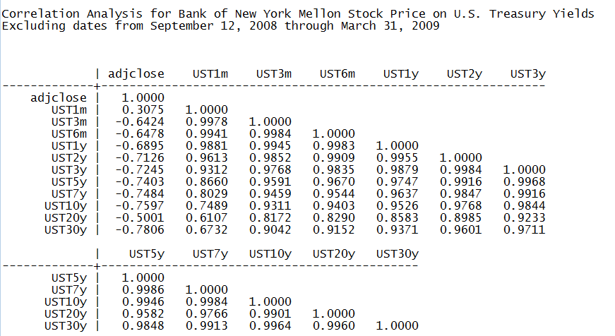
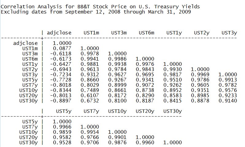
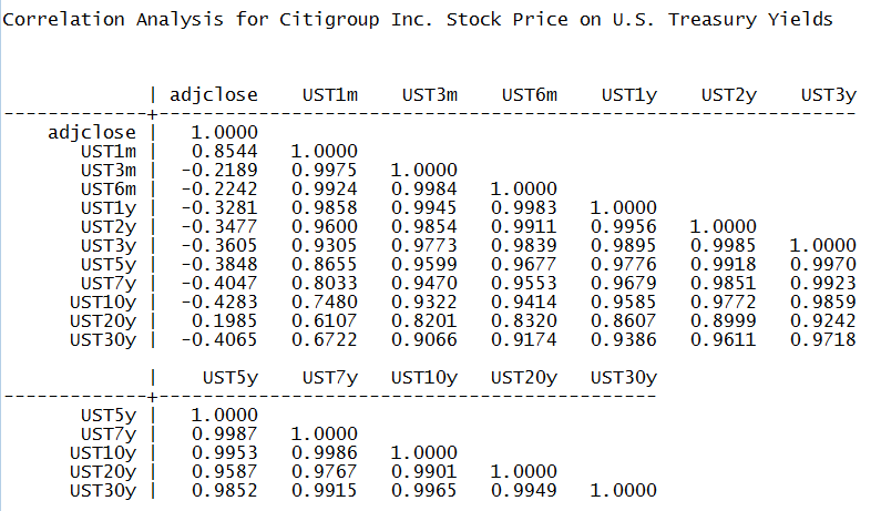
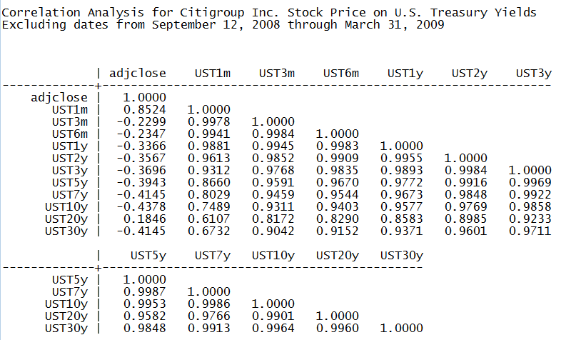
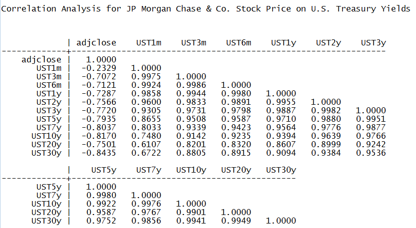
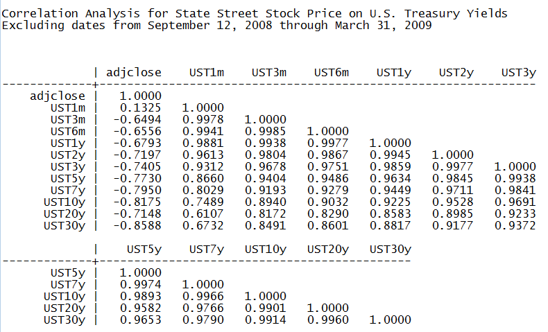
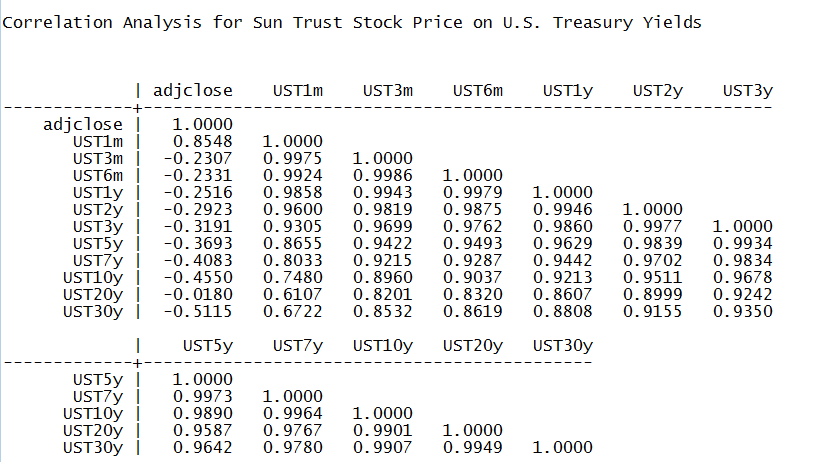
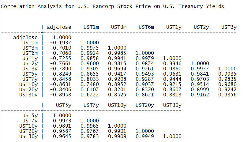
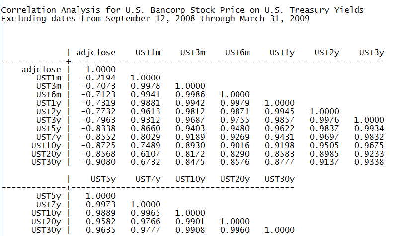
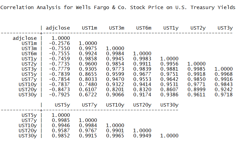
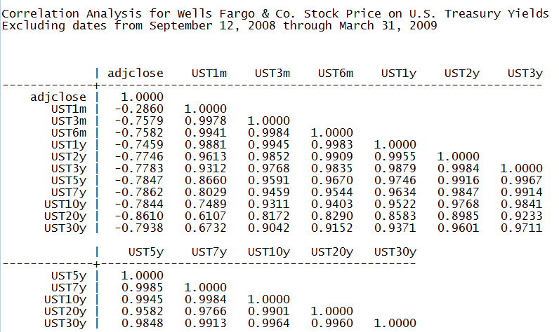
We want to thank our readers for the very strong response to our June 17, 2015, note “Bank Stock Prices and Higher Interest Rates: Lessons from History.” For those readers who asked “is the correlation between Treasury yields and bank stock prices negative at other maturities besides the 10 year maturity?” – we include Appendix A. Appendix A shows that for all nine bank holding companies studied, there is negative correlation between the bank’s stock price and Treasuries for all maturities but two. One exception is the 1-month Treasury bill yield, which is the shortest time series reported by the U.S. Department of the Treasury. The 1-month Treasury bill yield has only been reported since July 31, 2001. The correlation between the longer 3-month Treasury bill yield series and the stock prices of all nine bank holding companies is negative. The other series that occasionally has positive correlations is the 20 year U.S. Treasury yield, which is the second shortest yield series provided by the U.S. Department of the Treasury.
In this note, we use modern “no arbitrage” finance and a story from 1974 to explain why there is and there should be a negative correlation between bank stock prices and interest rates. We finish with recommendations for further reading for readers with a very strong math background.
Wm. Mack Terry and Lessons from the Bank of America, 1974
In the summer of 1974 I began the first of two internships with the Financial Analysis and Planning group at Bank of America (NYSE:BAC) in San Francisco. My boss was Wm. Mack Terry, an eccentric genius from MIT and one of the smartest people ever to work at the Bank of America. One day he came to me and made a prediction. This is roughly what he said:
“Interest rates are going to go up, and two things are going to happen. Our net income and our net interest margins are going to go up, and our senior management is going to claim credit for this. But they’ll be wrong when they do so. Our income will only go up because we don’t pay interest on our capital. Shareholders are smart and recognize this. When they discount our free cash flow at higher interest rates, even with the increase on capital, our stock price is going to go down.”
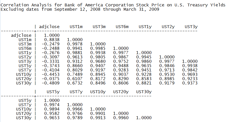
Everything Mack predicted came true. The 1-year U.S. Treasury yield was in the 8 percent range in the summer of 1974. It ultimately peaked at 17.31% on September 3, 1981. The short run impact of the rate rise was positive at Bank of America, but the long run impact was devastating. By the mid-1980s, the bank was in such distress that my then employer First Interstate Bancorp launched a hostile tender to buy Bank of America.
The point of the story is not the anecdote about Bank of America per se. Why was Mack’s prediction correct? We give the formal academic references below, but we can use modern “no arbitrage” financial logic to understand what happened. We model a bank that’s assumed to have no credit risk by replication, assembling the bank piece by piece from traded securities. This was the approach taken by Black and Scholes in their famous options model, and it’s a common one in modern “no arbitrage” finance. We take a more complex approach in the “Technical Notes” section. For now, let’s make these assumptions to get at the heart of the issue:
- We assume the bank has no assets that are at risk of default.
- All of its profits come from investing at rates higher than U.S. Treasuries and by taking money from depositors at rates lower than U.S. Treasury yields
- We assume that the bank borrows money in such a way that all assets financed with borrowed money have no interest rate risk: the credit spread is locked in. We assume the net interest margin is locked in at a constant dollar amount that works out to $3 per share per quarter.
- We assume this constant dollar amount lasts for 30 years.
- With the bank’s capital, we assume the bank either buys 3-month Treasury bills or 30-year fixed rate Treasury bonds. We analyze both cases.
- We assume taxes are zero and that 100% of the credit spread cash flow is paid out as dividends to keep things simple.
- We assume the earnings on capital are retained and grow like the proceeds of a money market fund.
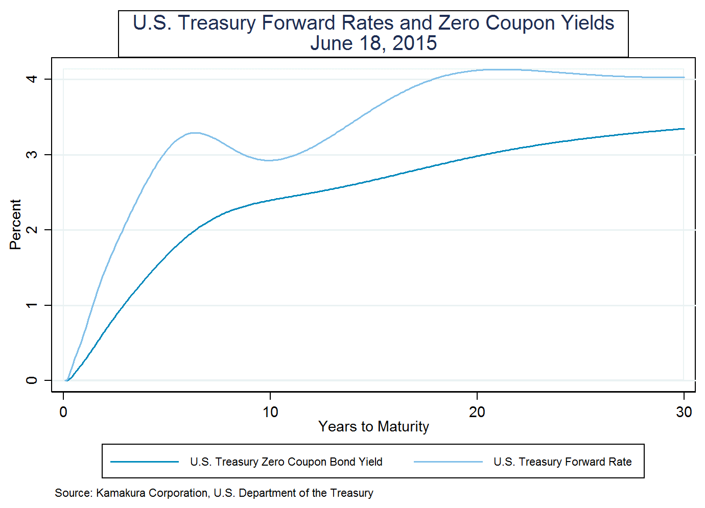
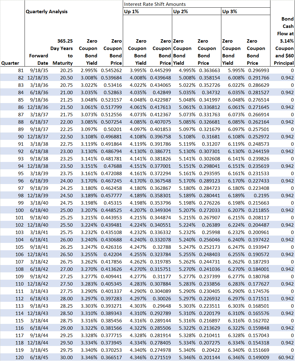
We use the U.S. Treasury curve of June 18 to analyze our simple bank. The present value of a dollar received in 3 months, 6 months, 9 months, etc. out to 30 years can be calculated using U.S. Treasury strips (zero coupon bonds) whose yields are shown here:
(click to enlarge)
We write the present value of a dollar received at time tj as P(tj). The first quarter is when j is 1. The last quarter is when j is 120. The cash flow thrown off to shareholders from the hedged borrowing and lending is the sum of $3 per quarter times the correct discount factors out to 30 years.
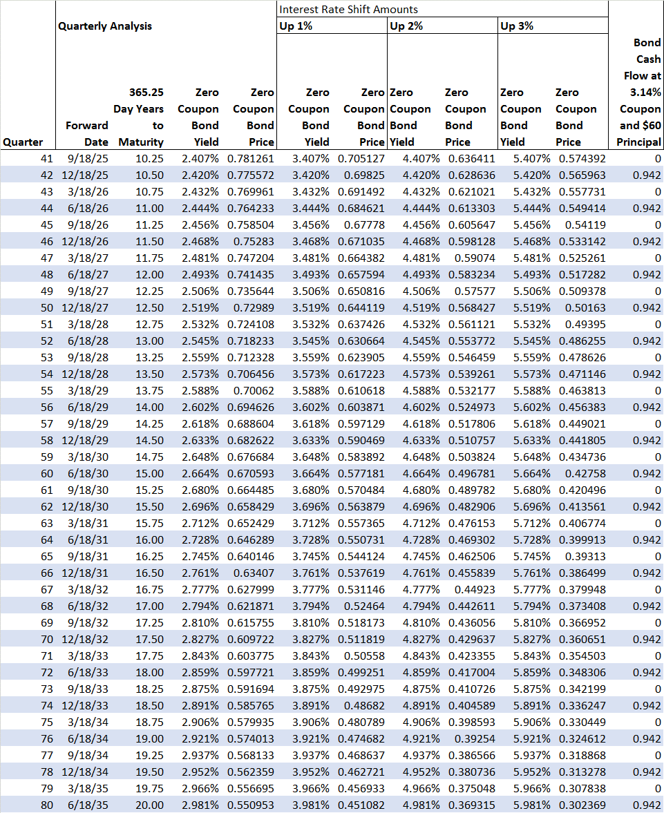
The sum of the discount factors is 81.02. When we say “the sum of the discount factors,” note that means that the entire 30 year Treasury yield curve is used in valuing the bank’s franchise, even if the bank makes that $3 per quarter rolling over short term assets and liabilities. When we multiply the sum of the discount factors by $3 per quarter, the value of the hedged lending business contributes $3 x 81.02 = $243.06 to the share price. This calculation is given in Appendix B.
How about the value of earnings on capital? And how much capital is there? The short answer is that it doesn’t matter – we’re just trying to illustrate valuation principals here. But let’s assume the $3 in quarterly “spread” income, $12 a year, is 1% of assets. That makes assets $1200 (per share). With 5% capital, we’ll use $60 as the bank’s capital. We analyze two investment strategies for capital: Strategy A is to invest in 3-month Treasury bills. They are yielding 0.01% on June 18. Strategy B is to invest in the current 30 year Treasury bond, yielding 3.14% on June 18. Let’s evaluate the stock price right now under both strategies. If rates don’t move, the current outlook is this if the bank invests its capital in Treasury bills using Strategy A:

Net income will be $12.006 per year. The value of capital at time zero is $60 because we’ve invested $60 in T-bills worth $60. The value of the hedged “spread lending” franchise, discounted over its 30-year life, is $243.060. That means the stock price must be the sum of these two pieces or there’s a chance for risk-less arbitrage. The stock price must be $303.060.
What happens to the stock price if, one second after we buy the stock, zero coupon bond yields across the full yield curve rise by 1%, 2%, or 3%? This is a mini-version of the Federal Reserve’s Comprehensive Capital Analysis and Review stress tests. The stock price changes like this:

Higher rates are “good for the bank” in the sense that net income will rise because earnings on the 3-month Treasury bills will be 1%, 2% or 3% higher. This is exactly what Mack Terry explained to me in 1974. This has no impact on stock price, however, because the investment in T-bills is like an investment in a money market fund. Since the discount factor rises when the income rises, the value is stable. So the value of the invested capital is steady at $60. See the “Technical Notes” references for background on this. What happens to the value of the spread lending franchise? It gets valued just like a constant payment mortgage that won’t default or prepay. The value drops from $243.06 to either $215.04, $191.55 or $171.72. The calculations also are given in Appendix B. The result is a stock price that’s lower in every scenario, dropping 9.25%, 17.00% or 23.54%.
But wait, one might ask. Won’t the amount of lending increase and credit spreads widen at higher rates? Before we answer that question, we can calculate our breakeven expansion requirements. For the value of the lending franchise to just remain stable, we need to restore the value from 215.04, 191.55 or 171.72 to 243.06. This requires that the cash flow expand by 243.06/215.04-1 in the “up 1%” scenario. That means our cash flow has to expand by 13.03% from $12 a year to $13.56 per year. For the up 2% and up 3% scenarios, the increases have to be by 26.89% or 41.54%.
Just from a common sense point of view, this expansion of lending volume seems highly unlikely at best. A horde of academic studies discussed in Chapter 17 of van Deventer, Imai and Mesler also have found that when rates rise, credit spreads shrink rather than expand. Selected references are given in the “Technical Notes.”
Is Strategy B a better alternative? Sadly, no, because the income on invested capital stays the same (3.14% times $60) and the present value of the 30-year bond investment falls. Here are the results:

Good News and Conclusions
There is some good news in this analysis. Given the assumptions we have made, this bank will never go bankrupt. Because the assets funded with borrowed money are perfectly hedged from a rate risk point of view, the bank is in the “safety zone” that Dr. Dennis Uyemura and I described in our 1992 introduction to interest rate management, Financial Risk Management in Banking. The other good news is that Mack Terry’s example shows that the entire spectrum of Treasury yields is used to value bank stocks because the cash flow stream from the banking franchise spans a 30-year time horizon.
This example shows that, under simple but relatively realistic assumptions, the value of a bank can be replicated as a portfolio of Treasury-related securities. This portfolio falls in value when rates rise. The negative correlation between Treasury yields that 30 years of history shows is not spurious correlation – it’s consistent with the fundamental economics of banking when interest rate risk is hedged.
Wm. Mack Terry knew this in 1974, and legions of interest rate risk managers of banks have replicated this simple example in their regular interest rate risk simulations that are required by bank regulators around the world. What surprises me is that people are surprised to learn that higher interest rates lower bank stock prices.
Technical Notes
When writing for a general audience, some readers become concerned that the author only knows the level of analysis reflected in that article. We want to correct that impression in this section. We start with some general observations and close with references for technically oriented readers:
- For more than 50 years, beginning with the capital asset pricing model of Sharp, Mossin and Lintner, securities returns have been analyzed on an excess return basis relative to the risk free rate as a function of one or more factors. It is well known that the capital asset pricing model itself is not a very accurate description of security returns as a function of the risk factors.
- Arbitrage pricing theory expanded explanatory power by adding factors. Merton’s inter-temporal capital asset pricing model (1974) added interest rates driven by one factor with constant volatility.
- Best practice in modeling traded asset returns is defined by Amin and Jarrow (1992), who build on the multi-factor Heath, Jarrow and Morton interest rate model which allows for time varying and rate varying interest rate volatility. Amin and Jarrow also allow for time varying volatility as a function of interest rate and other risk factors.
- This is the procedure my colleagues and I use to decompose security returns. An important part of that process is an analysis of credit risk, as explained by Campbell, Hilscher and Szilagyi (2008, 2011). Jarrow (2013) explains how credit risk is incorporated in the Amin and Jarrow framework. This is the procedure we would explain in a more technical forum, like our discussion with clients.
- Asset return analysis is built on the Heath Jarrow and Morton interest rate simulation. The most recent 100,000 scenario simulation for U.S. Treasury yields (“The 3 Month T-bill Yield: Average of 100,000 Scenarios Up to 3.23% in 2025“) was posted on Seeking Alpha on June 16, 2015.
References for random interest rate modeling are given here:
Heath, David, Robert A. Jarrow and Andrew Morton, “Bond Pricing and the Term Structure of Interest Rates: A Discrete Time Approach,” Journal of Financial and Quantitative Analysis, 1990, pp. 419-440.
Heath, David, Robert A. Jarrow and Andrew Morton, “Contingent Claims Valuation with a Random Evolution of Interest Rates,” The Review of Futures Markets, 9 (1), 1990, pp.54 -76.
Heath, David, Robert A. Jarrow and Andrew Morton,”Bond Pricing and the Term Structure of Interest Rates: A New Methodology for Contingent Claim Valuation,” Econometrica, 60(1), 1992, pp. 77-105.
Heath, David, Robert A. Jarrow and Andrew Morton, “Easier Done than Said”, RISK Magazine, October, 1992.
References for modeling traded securities (like bank stocks) in a random interest rate framework are given here:
Amin, Kaushik and Robert A. Jarrow, “Pricing American Options on Risky Assets in a Stochastic Interest Rate Economy,” Mathematical Finance, October 1992, pp. 217-237.
Jarrow, Robert A. “Amin and Jarrow with Defaults,” Kamakura Corporation and Cornell University Working Paper, March 18, 2013.
The impact of credit risk on securities returns is discussed in these papers:
Campbell, John Y., Jens Hilscher and Jan Szilagyi, “In Search of Distress Risk,” Journal of Finance, December 2008, pp. 2899-2939.
Campbell, John Y., Jens Hilscher and Jan Szilagyi, “Predicting Financial Distress and the Performance of Distressed Stocks,” Journal of Investment Management, 2011, pp. 1-21.
The behavior of credit spreads when interest rates vary is discussed in these papers:
Campbell, John Y. & Glen B. Taksler, “Equity Volatility and Corporate Bond Yields,” Journal of Finance, vol. 58(6), December 2003, pages 2321-2350.
Elton, Edwin J., Martin J. Gruber, Deepak Agrawal, and Christopher Mann, “Explaining the Rate Spread on Corporate Bonds,” Journal of Finance, February 2001, pp. 247-277.
The valuation of bank deposits is explained in these papers:
Jarrow, Robert, Tibor Janosi and Ferdinando Zullo. “An Empirical Analysis of the Jarrow-van Deventer Model for Valuing Non-Maturity Deposits,” The Journal of Derivatives, Fall 1999, pp. 8-31.
Jarrow, Robert and Donald R. van Deventer, “Power Swaps: Disease or Cure?” RISK magazine, February 1996.
Jarrow, Robert and Donald R. van Deventer, “The Arbitrage-Free Valuation and Hedging of Demand Deposits and Credit Card Loans,” Journal of Banking and Finance, March 1998, pp. 249-272.
The use of the balance of the money market fund for risk neutral valuation of fixed income securities and other risky assets is discussed in technical terms by Heath, Jarrow and Morton and in a less technical way:
Jarrow, Robert A. Modeling Fixed Income Securities and Interest Rate Options, second edition, Stanford Economics and Finance, Stanford, 2002.
Jarrow, Robert A. and Stuart Turnbull, Derivative Securities, second edition, South-Western College Publishing, 2000.
Appendix A: Expanded Correlations
The expanded correlations in this appendix use data from the U.S. Department of the Treasury as distributed by the Board of Governors of the Federal Reserve in its H15 statistical release.
It is important to note that the 1-month Treasury bill rate has only been reported since July 31, 2001, and that is the reason that the correlations between bank stock prices and that maturity are so different from all of the other maturities. The history of reported data series is taken from van Deventer, Imai and Mesler, Advanced Financial Risk Management, 2nd edition, 2013, chapter 3.
(click to enlarge)
Bank of America Corporation Correlations
(click to enlarge)
(click to enlarge)
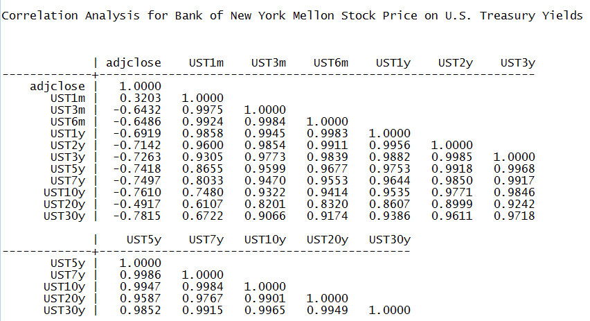
Bank of New York Mellon Correlations
(click to enlarge)
(click to enlarge)
BB&T Correlations
(click to enlarge)
(click to enlarge)
Citigroup Inc. Correlations
(click to enlarge)
(click to enlarge)
JP Morgan Chase & Co. Correlations
(click to enlarge)
(click to enlarge)
State Street Correlations
(click to enlarge)
(click to enlarge)
Sun Trust Correlations
(click to enlarge)
(click to enlarge)
U.S. Bancorp Correlations
(click to enlarge)
(click to enlarge)
Wells Fargo & Company Correlations
(click to enlarge)
(click to enlarge)
Appendix B
Valuing the Banking Franchise: Worked Example
The background calculations for today’s analysis are given here. The extraction of zero coupon bond prices from the Treasury yield curve is discussed in van Deventer, Imai and Mesler (2013), chapters 5 and 17.
(click to enlarge)
(click to enlarge)
(click to enlarge)